The inception of this study was the resolution of a production challenge involving interpretation constructions using a complex of geophysical and associated methods, performed with unmanned aerial vehicles and payloads manufactured by the Geoscan company of Russia. This paper explores methods to enhance the geological significance of interpretive recalculations within the complex of the anomalous magnetic field, the absolute height field of the digital elevation model, and the halftone field of photo anomalies in a multichannel remote sensing framework. The objective of this study is to develop filtering methods and depth parametric recalculations, which are invariant to the type of geofield being processed.
- Introduction
- Methodology of field and office investigations
- Comprehensive geological and geophysical interpretation
- Conclusion
Introduction
As of today, the application of unmanned aerial vehicles (UAVs) for civilian purposes has a long history both in Russia and worldwide. In Russia, several leading organizations conduct UAV surveys for geological exploration purposes.
This study uses data gathered from a survey executed by the Geoscan Group of Companies, a leading Russian entity in UAV technology deployment for geological exploration, during the 2022 field season.
The paper examines a promising site in the Lovozero district of the Murmansk region as the study area. The ore occurrence under consideration, located in the upper reaches of the Teriberka River, consists of a family of coulisse-like lenses of dipyroxene-magnetite quartzites ranging up to 100-140 meters in thickness and extending from 100 meters to 1.5 km, with the depth of the magnetite and hematite-magnetite ores estimated up to 500 meters. The ore node, along with the Central Kola and Sholtyarvi ore clusters, is part of the Central Kola iron ore metallogenic zone (MZ). In its formation area, deposits of ferruginous quartzites tend to align with linear suture structures, remnants of Archean greenstone belts, and are also found in narrow depressions surrounded by granite-gneiss domes. In the vicinity of the licensed area, crystalline complexes have developed, the contact surfaces of which extend in a northwestern azimuth. In this context, the intersection area of two regional faults – a discordant structure with northeastern and submeridional orientations, lying within the licensed boundaries – is delineated. The spatial association of the study area with the discordant structure suggests the potential manifestation of ring structure markers in the morphology of the measured geofields, centered in the noted intersection area of regional faults.
The structure of the Central Kola MZ, to which the examined deposit is associated, features a flattened configuration of tonalite lenses, extending to a strata-like form. Most ore occurrences consist of alternating "layers" of tonalite gneisses and crystalline schists, containing lenses of ferruginous quartzites. Another characteristic of the Central Kola MZ is a significant portion of complexes metamorphosed under granulite facies conditions, with a complete absence of not only large deposits but also large ore bodies. In most sections, primary crystalline schists dominate, though they are practically absent in the ore occurrences of this area, where ferruginous quartzites lie within biotite and alumina gneisses.
Methodology of field and office investigations
The study area covers approximately 30 square kilometers, making the conduct of ground-based geophysical surveys challenging. As a result, it was decided to carry out the work using such equipment as lightweight and compact drones with various payloads.
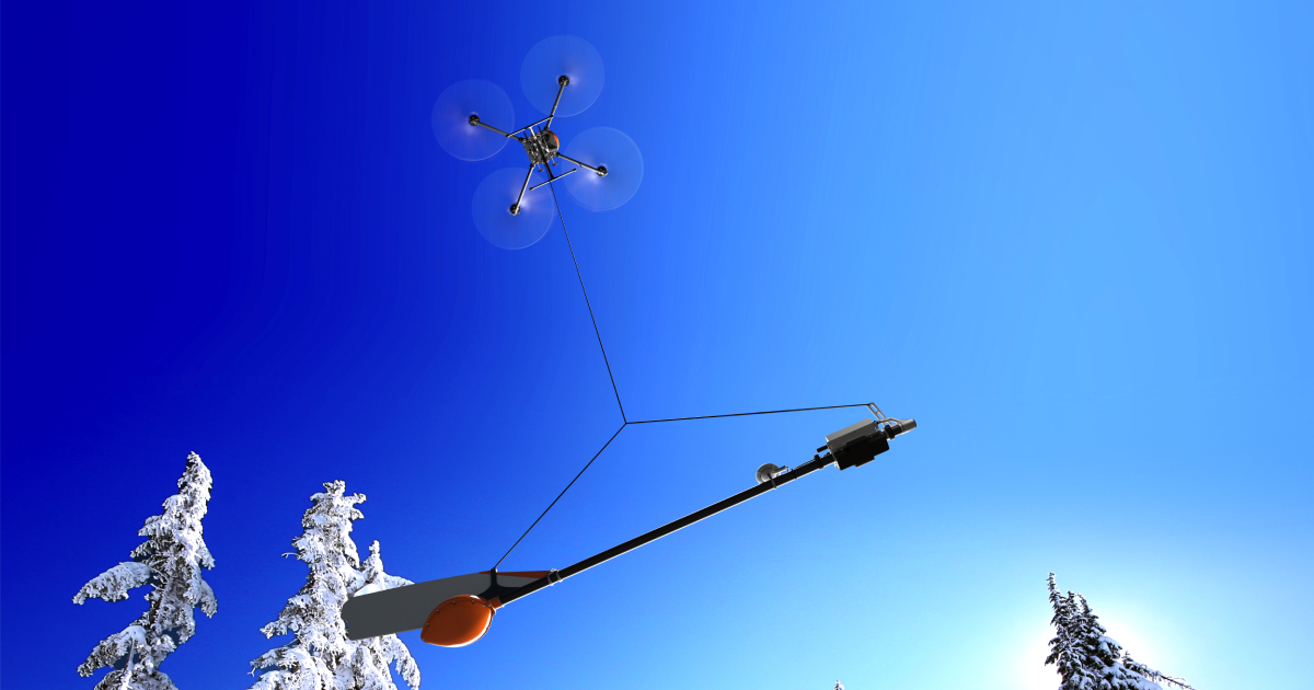
A range of activities was conducted at the site, including aeromagnetic surveying using UAVs, along with aerial photogrammetric surveying and scanning of local relief forms. All work was conducted by the Geoscan Group using their equipment and personnel. Initially, aerial photography is performed to create an elevation map, facilitating subsequent UAV flights that closely follow the terrain contours. The aeromagnetic survey employs the Geoscan 401 Geophysics system, comprising a lightweight multi-rotor quadcopter and a Geoscan GeoShark quantum magnetometer mounted on the drone. Flights for aeromagnetic surveying are conducted at the lowest feasible altitude. This aspect is crucial as maintaining the specified condition minimizes the sensor's distance from the mountain massif, allowing for the capture of a higher quality signal that is not overshadowed by signals from larger objects.
Standard office processing of field magnetic survey results using UAVs involves sequential execution of the following operations: adjusting for daily variations of the Earth's geomagnetic field; correcting for the Earth's normal field; correlating reference and series routes; and estimating the standard deviation.
The primary goal of processing aeromagnetic survey data is to generate a digital model of the anomalous magnetic field in the survey area, assess the accuracy of the obtained measurements, and create maps of the anomalous magnetic field and transformation maps (Fig. 1).
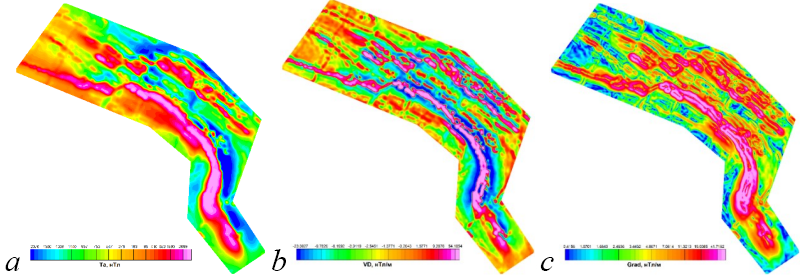
Figure 1. Maps of the surveyed area, derived from field aeromagnetic work with UAVs and office processing:
a. Anomalous magnetic field map;
b. Map of the vertical derivative of the anomalous magnetic field;
c. Map of the total horizontal gradient of the anomalous magnetic field
Comprehensive geological and geophysical interpretation
Moving on to quantitative and qualitative geological and geophysical interpretation, we would like to highlight the main sequence of actions, which will be detailed further below:
- Step-by-step morphostructural reconstruction of ore-controlling factors based on the interpretation of remote sensing data. The reconstruction involves lineament interpretation of remote sensing imagery at various scale levels, resulting in a generalized image of the ore-controlling structure.
- Adjustment of the anomalous magnetic field for local relief forms followed by verification and refinement of the remote sensing interpretation results, using automated interpretation technology of the anomalous magnetic field.
- Optimal filtration of the anomalous magnetic field to localize responses as intense strip anomalies, spatially correlated with the location of ferruginous quartzites.
- Calculation of the geoblock structure of the area by transforming the anomalous magnetic field into a scalar field of spatial stationarity parameter values.
- Employing reduction of the anomalous magnetic field and subsequent adjustment for local landforms, an analytical continuation is performed from the observation surface to the volume of the rock massif.
- The final outcome of these transformations is a comprehensive forecast scheme, where updated elements (new predictive contours of ore bodies) are laid out on pre-defined contours (of ore bodies and projections of contact surfaces onto the cartographic plane).
The remote sensing data is represented by a grayscale infrared channel, used in processing to register the ore-controlling structure, which is evident over an area larger than the licensed area. Regarding the remote sensing data, the following procedures are conducted: enhancement of overall contrast through brightness distribution histogram normalization; edge detection of extended elements (lineaments) using the Sobel operator; GRB combination with the digital elevation model and regional magnetic field; and contrasting of linearized structures based on tracing the identified linear contours with isolines.
The result of this procedure is the localization of distinct lineament structures, within whose system the pattern of spatial distribution of ore objects may be identified (Fig. 2). Overlaying the reconstruction of the first-order structural plan on pre-defined elements of the geological base reveals: a distinct localization of the discordant structure in the area of a coulisse-like bend of known ore body contours; the clustering of known ore mineralization points coincides with the discordant structure's localization and the center of a zircoid structure, likely indicating processes of stage-by-stage vertical movements in relation to the area of maximum permeability of the rock massif (discordant structure); elements of the first-order structural plan correlate unambiguously with the pre-defined set of disjunctive features; fragmented strip zones, correlating with contours of known ore objects, are identified within the system of radial faults.
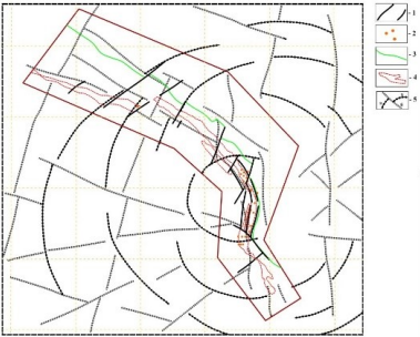
Figure 2. Reconstruction of ore-controlling elements in the first-order structural plan. Legend:
1. Pre-defined elements of geological fracturing;
2. Pre-defined and verified points of ore mineralization;
3. Pre-known projection on the cartographic plane of the contact surface between volcanogenic and volcanogenic-terrigenous formations;
4. Contours of ore bodies;
5. Reconstruction of the first-order structural plan (a. zircoid formation; b. radial disjunctives controlling known ore objects)
In processing the anomalous magnetic field, let us first assess its functional relationship with the local forms of the Earth's surface relief. This assessment is aimed at incorporating corrections into the structure of the anomalous magnetic field to exclude responses from local landforms. The importance of these corrections lies in the disassembly or verification of the lineament image obtained from the remote sensing data, through its comparison with the deep (endogenous) geostructural image derived from magnetic field analysis, as well as ensuring quantitative recalculations of the anomalous magnetic field from a flat surface parallel to the geoid surface.
To conduct the aforementioned assessment, we calculate the pair correlation coefficient between the anomalous magnetic field and the field of absolute heights of the Earth's surface relief. The pair correlation coefficient |r(Ta,Rel)|=0.21<0.5, indicates a weak linear relationship between the magnetic field and local land surface relief forms. Nonetheless, to ensure the complete absence of functional dependence between the anomalous magnetic field Ta and local landforms R, we derive a linear function of the following form:
Ta = -4443.814+16.394 * R ,
based on which, for any value of R, we calculate the component of the anomalous magnetic field δTa, caused by local relief forms R. Subtracting δTa from the actual anomalous magnetic field data results in a zero pair correlation coefficient between Та and R.
Let us perform tracing of geostructural axes in the magnetic field after applying the δТа correction. The basis of constructing geostructural axes is the recalculation of the areal distribution of anomalous magnetic field values into the curvature parameter of the virtual (magnitude) surface of this field, expressed in the direction of the magnetic field gradient vector, wherever this field is defined. Negative curvature, shown in Fig. 4, a with dark gray shading, indicates an antiform in the structure of the virtual surface of the field.
Using halftone shading of the isoline parameter K scheme, and excluding the image of the isolines themselves, results in a spatial scheme of geostructural axes that intricately maps linear and nonlinear structural elements, shear kinematics, and local areas of discordant intersections. Combining the remote sensing data transformants and the endogenous geostructural plan allows us to reconstruct elements of the 2nd order geostructural image, subordinate to the 1st order geostructural image.
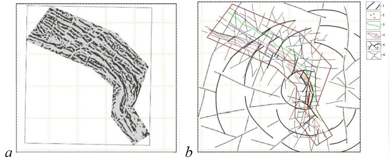
Figure 3. Reconstruction of the 2nd order geostructural plan and its integration with the 1st order geostructural plan:
a. Transformation of the digital model of the anomalous magnetic field into the geostructural image of the license area;
b. Joint interpretation of the transformant in Fig. 5.9., "a" and the remote sensing data transformant in Fig. 5.4., resulting in a consolidated geostructural image of the study area (in the legend: 5 – elements of the 1st order geostructural image; 6 – the same for the 2nd order);
Overlaying the final geostructural scheme with pre-defined elements of the large-scale geological base suggests the presence of two fragmented band zones controlling the development of desired ore objects: one band zone confirms the position of known ore contours; the other is situated further north and leans towards the volcanogenic formation.
The next step in processing the anomalous magnetic field involves localizing anomalous zones directly associated with standards. To achieve this, a low-pass filtering approach is implemented. The comparison between the a priori known geological base, the primary image of the anomalous magnetic field (Fig. 4, a), and the filtering result (Fig. 4, b) demonstrates that responses from the contact surface of volcanogenic and volcanogenic-terrigenous formations in the anomalous magnetic field are weakly expressed and are smoothed against the background of intense anomalies generated by ferruginous quartzites; south of this contact surface's projection on the map plane, there is a series of banded positive magnetic anomalies that confirm the a priori defined ore body contours; north of this projection, there is a highly fragmented series of positive anomalies, which, as noted earlier, are of an intensity comparable to anomalies characteristic of the northern part of the a priori known ore body contours.
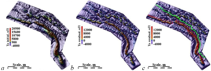
Figure 4. The result of optimal filtering of the anomalous magnetic field:
a. Contrasted image of the anomalous magnetic field;
b. High-frequency component of the anomalous magnetic field;
c. Superimposition in Fig. 4, b of the a priori known ore body contours (red dashed line) and the contact between structural-compositional complexes (SCCs) (green line)
The calculation of the spatial stationarity parameter (Fig. 5) contrasts the intense positive magnetic anomaly families located north of the contact between volcanogenic and volcanogenic-terrigenous SCCs.
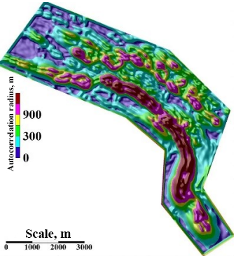
Figure 5. Distribution of the spatial stationarity parameter of the anomalous magnetic field, highlighting the zonality within the area
In the three-dimensional quantitative interpretation of the anomalous magnetic field, it is important to note that the work focused exclusively on its residual component: the downward recalculation was conducted from a hypothetical flat observation surface; intense extremes in the structure of the anomalous magnetic field, which overshadow other features and are associated with the influence of ore bodies, are observed in a narrow depth range and lose their distinct configurations as the recalculation depth increases, indicating a move beyond the boundary of the anomaly-forming source.
The downward recalculation is based on a known sequence of operations as the depth increases: conversion of the anomalous magnetic field into the Fourier spectrum; contrasting of spectral harmonics related to the determined depth of the analytical continuation of the anomalous magnetic field; conversion of the transformed Fourier spectrum back to the object plane, obtaining an image of the anomalous magnetic field at a fixed depth; subtracting this field image from the original magnetic field.
The outcome of the recalculation is a series of horizontal cross-sections of the three-dimensional block-diagram of the rock massif, each section representing the distribution pattern of the intensity of the anomalous magnetic field image characteristic of a specified depth. This recalculation can reveal the depth at which the magnetized ore fraction (here, the zones of ferruginous quartzite formation) exhibits its maximum manifestation, marked by local intensive responses. As shown in the three cross-sections in Fig. 6, up to a depth of about 50 meters, a highly differentiated structure of intense strip magnetic anomalies is observed both in the region of a priori known ore contours and to their north.
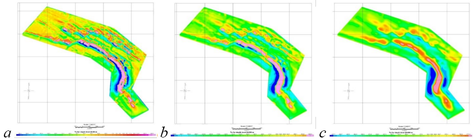
Figure 6. Results of the analytical recalculation of the magnetic field to depth:
a. 50 m;
b. 200 m;
с. 500 m
Conclusion
Therefore, from the foregoing, it can be inferred that at a depth of 200 meters, a significant smoothing of the contours of intense magnetic anomalies occurs, suggesting that this depth exceeds the boundaries of the localization area for key points (the upper and lower margins of the anomaly-generating object). At a depth of 500 meters, only trend traces of anomalous zones are observed, suggesting that the 500-meter mark represents the boundary for the formation of traceable ore bodies.
Summarizing the above findings, the northern group of strip magnetic anomalies (Fig. 7) is identified as predictive for the formation of ferruginous quartzites.
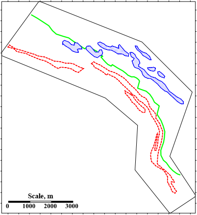
Figure 7. The predicted zone, shown against the background of a priori defined elements of the large-scale geological base:
Blue indicates the predicted zone;
Red indicates the contours of ore bodies;
Green marks the contact of volcanogenic and volcanogenic-terrigenous formations.
In the northwestern part of the prospective objects highlighted in (Fig. 7), their proximity to the contact of volcanogenic-terrigenous and volcanogenic SCCs is observed. Moving eastward, the predicted strip zone shifts northward relative to the marked contact, exhibiting more pronounced segmentation along the plane of disjunctives with shear kinematics than in the a priori defined ore contours. The structure of the predicted strip zone includes echelonization – the presence of subparallel strip formations, whose thickness diminishes as they extend from southwest to northeast.
References to sources used in the article have been removed. List of references is available in the original publication.
Authors of the article: Z.I. Sadykova, I.B. Movchan, A.A. Yakovleva, D.A. Goglev.
Published in the Geology and Mineral Resources of the Western Urals scientific journal, 2023. № 6 (43), pages 161–169.